

A Gaussian distribution is also called:
Gaussian Distribution = Normal Distribution = Bell-Shaped Distribution
They all mean the same thing.
1. What Is a Gaussian Distribution?
A Gaussian distribution describes data where:
Most values are close to the average, while values become less common as we move farther away from the average.
For example, imagine the heights of thousands of people.
Most people may be close to the average height.
Very short people are less common.
Very tall people are also less common.
The graph often looks like this:
Probability
    ^
    |
    |                 ***
    |              *********
    |            *************
    |          *****************
    |       ************************
    |____******************************____
         short     average       tall
                      μ
This is why it is called a bell-shaped curve.
2. The Two Most Important Parameters
A Gaussian distribution is mainly controlled by two values:
μ  = mean
σ  = standard deviation
And:
σ² = variance
The easiest way to remember them is:
μ = Where is the center?

σ = How wide is the distribution?

σ² = Variance
3. Understanding μ — The Mean
The Greek letter:
μ
is pronounced:
mu
It represents the average value.
Suppose we have:
10, 12, 14, 16, 18
The mean is:
μ = (10 + 12 + 14 + 16 + 18) / 5
So:
μ = 70 / 5
μ = 14
The Gaussian curve will therefore be centered at 14.
                /\
              /    \
            /        \
__________/____________\__________
             μ = 14
So:
μ controls the position of the Gaussian curve.
4. Understanding σ — Standard Deviation
Sigma:
σ
is the standard deviation.
It tells us how spread out the values are around the mean.
Consider these two datasets.
Dataset A
48, 49, 50, 51, 52
Mean:
μ = 50
The values are very close together.
So sigma is small.
Small σ

               /\
              /  \
             /    \
____________/______\____________
               μ
Dataset B
20, 35, 50, 65, 80
The mean is still:
μ = 50
But the values are much more spread out.
Therefore sigma is larger.
Large σ

             ______
          __/      \__
       __/            \__
______/__________________\______
               μ
So:
Small σ = narrow distribution

Large σ = wide distribution
5. What Is Variance?
Variance is simply:
variance = σ²
For example:
σ = 2
Then:
σ² = 2²
σ² = 4
Another example:
σ = 0.5
Then:
σ² = 0.5²
σ² = 0.25
So remember:
σ  = standard deviation

σ² = variance
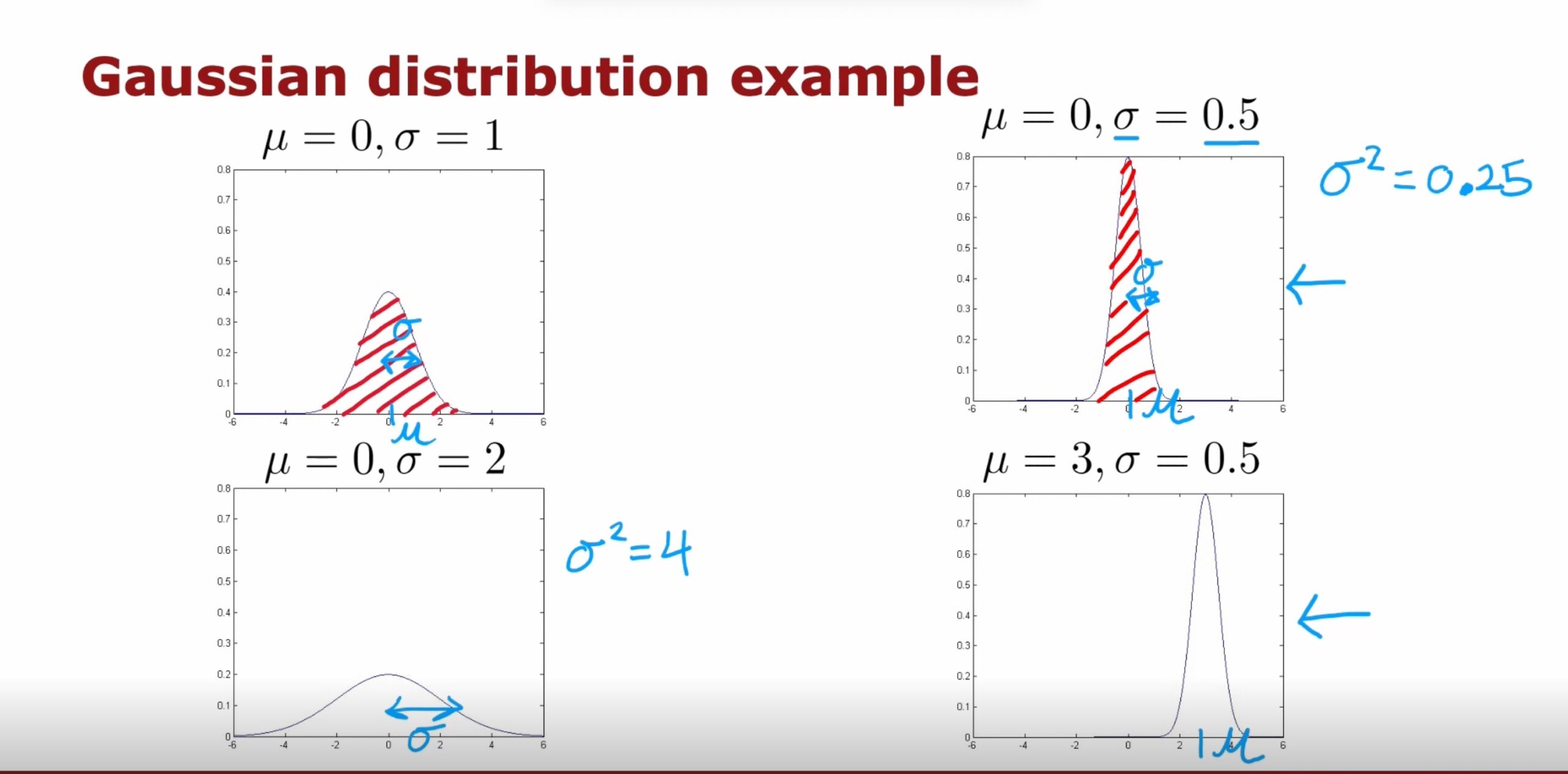
6. How μ and σ Change the Curve
Suppose:
μ = 0
σ = 1
The curve might look like:
                 /\
               /    \
             /        \
___________/____________\___________
                0
                μ
Now change sigma:
μ = 0
σ = 0.5
The curve becomes narrower and taller:
                  /\
                 /  \
                /    \
_______________/______\_______________
                  0
Now use:
μ = 0
σ = 2
The curve becomes wider and shorter:
              ________
           __/        \__
        __/              \__
_______/____________________\_______
                0
Now change the mean:
μ = 5
σ = 0.5
The curve moves to the right:
                            /\
                           /  \
__________________________/____\______
                           5
                           μ
Therefore:
| Parameter | Meaning |
|---|---|
| μ | Center of the curve |
| σ | Width or spread |
| σ² | Variance |
A useful rule is:
μ tells us where the bell is. σ tells us how wide the bell is.
7. Why Does a Narrow Gaussian Become Taller?
For a probability distribution, the total area under the curve must equal:
1
which means:
100% probability
So if the curve becomes narrower, it must become taller so that the total area remains 1.
Small σ                 Large σ

     /\                     ______
    /  \                 __/      \__
   /    \              _/            \_
__/______\__        ___/________________\___
Both curves still have total area:
1
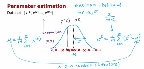
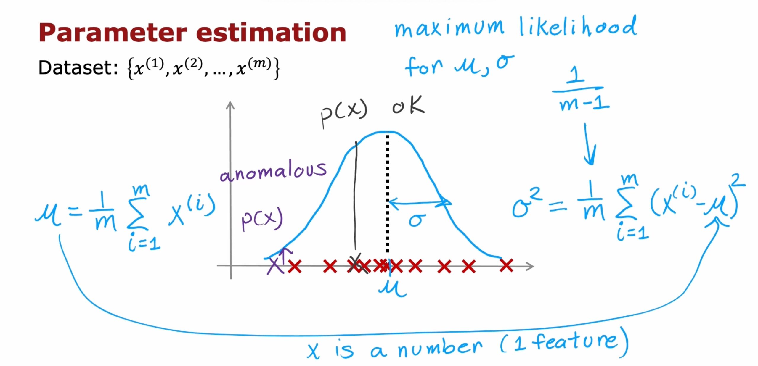
8. What Does p(x) Mean?
You will often see:
p(x)
In a Gaussian distribution, p(x) represents the probability density at the value x.
Imagine this curve:
                  *
                *   *
              *       *
            *           *
__________*_______________*__________
        A         B
Point B is near the center.
So:
p(B) = relatively high
Point A is far away from the center.
So:
p(A) = relatively low
This is the key idea behind anomaly detection.
Values near the center are usually common.
Values far away are usually unusual.
One technical detail:
p(x) is a probability density, not literally the probability that X equals exactly one value.
For continuous data, probability comes from the area under the curve across a range of values.
9. The Gaussian Formula
The Gaussian probability density function is:
             1
p(x) = --------------- × e ^ ( - (x - μ)² / (2σ²) )
       sqrt(2π) × σ
Another compact version is:
p(x) = [1 / (sqrt(2π) × σ)] × e^(-(x - μ)² / (2σ²))
Where:
x  = current value

μ  = mean

σ  = standard deviation

σ² = variance

π  ≈ 3.14159

e  ≈ 2.71828
You do not need to memorize this immediately.
The important part is:
(x - μ)
This means:
How far is x from the mean?
Then:
(x - μ)²
measures the squared distance from the mean.
If x is close to μ:
(x - μ)² is small
Therefore:
p(x) is relatively high
If x is far from μ:
(x - μ)² is large
Therefore:
p(x) becomes very small
This is why Gaussian distributions are useful for anomaly detection.
10. Calculating the Mean From Training Data
Suppose our training data is:
10, 12, 13, 14, 16
We have:
m = 5
The mean formula is:
μ = (1 / m) × Σ x(i)
In plain English:
Add all the values and divide by the number of examples.
So:
μ = (10 + 12 + 13 + 14 + 16) / 5
Therefore:
μ = 65 / 5
μ = 13
So the center of the Gaussian distribution is:
13
11. Calculating Variance
The variance formula is:
σ² = (1 / m) × Σ (x(i) - μ)²
In plain English:
- Take each value.
- Subtract the mean.
- Square the difference.
- Add the squared differences.
- Divide by the number of examples.
Using:
10, 12, 13, 14, 16
and:
μ = 13
we get:
| x | x – μ | (x – μ)² |
|---|---|---|
| 10 | -3 | 9 |
| 12 | -1 | 1 |
| 13 | 0 | 0 |
| 14 | 1 | 1 |
| 16 | 3 | 9 |
Add the squared differences:
9 + 1 + 0 + 1 + 9 = 20
Divide by 5:
σ² = 20 / 5
Therefore:
σ² = 4
To get standard deviation:
σ = sqrt(4)
Therefore:
σ = 2
So our Gaussian distribution has:
μ  = 13
σ  = 2
σ² = 4
12. How This Helps Detect Anomalies
Suppose normal server response times are:
100 ms
105 ms
110 ms
115 ms
120 ms
The mean is approximately:
110 ms
Now suppose a new request has response time:
112 ms
112 is close to the average.
Therefore:
p(112)
will likely be relatively high.
So we consider it normal.
Now suppose another request takes:
900 ms
900 ms is very far from the normal values.
Therefore:
p(900)
will be extremely small.
That suggests:
900 ms = possible anomaly
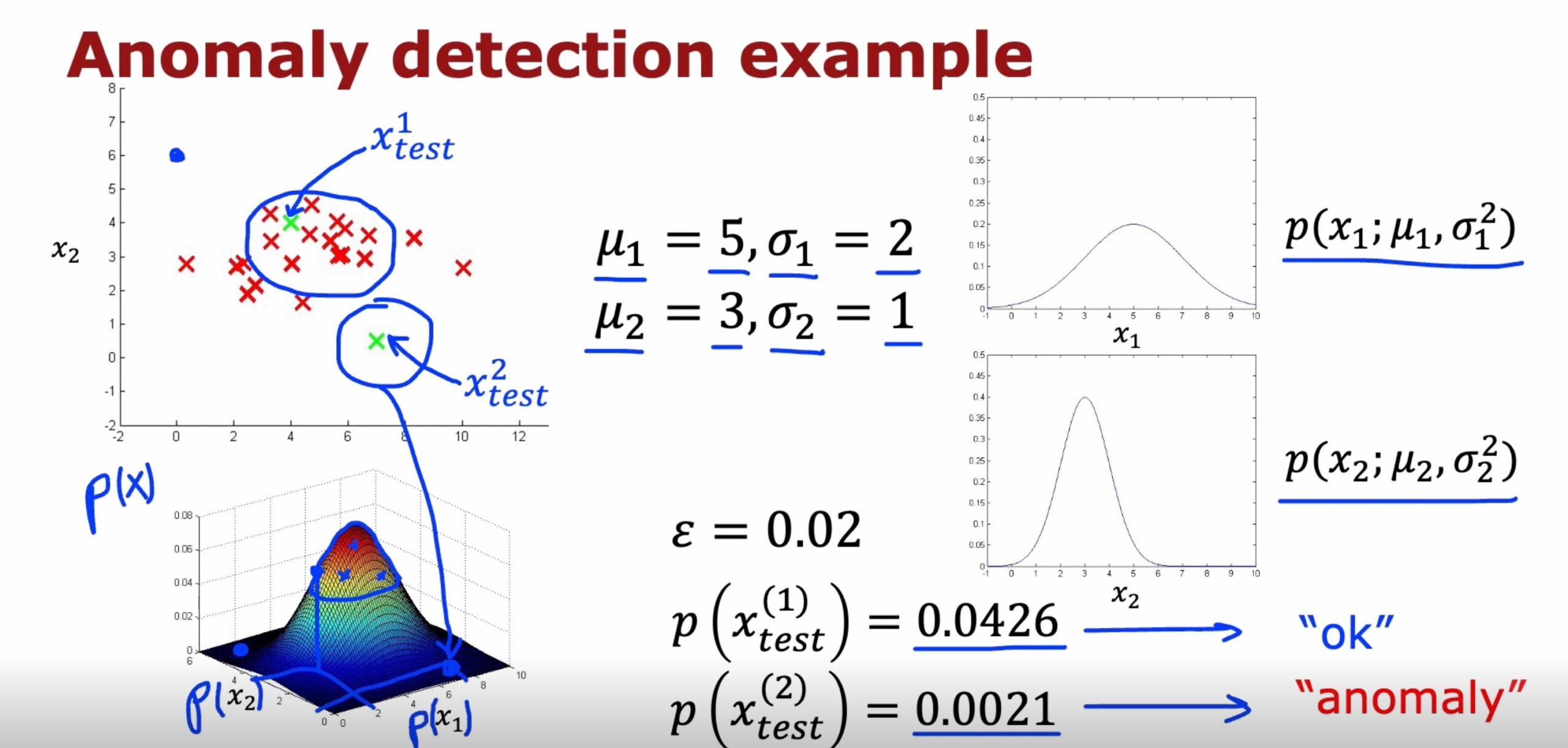
13. The Anomaly Threshold ε
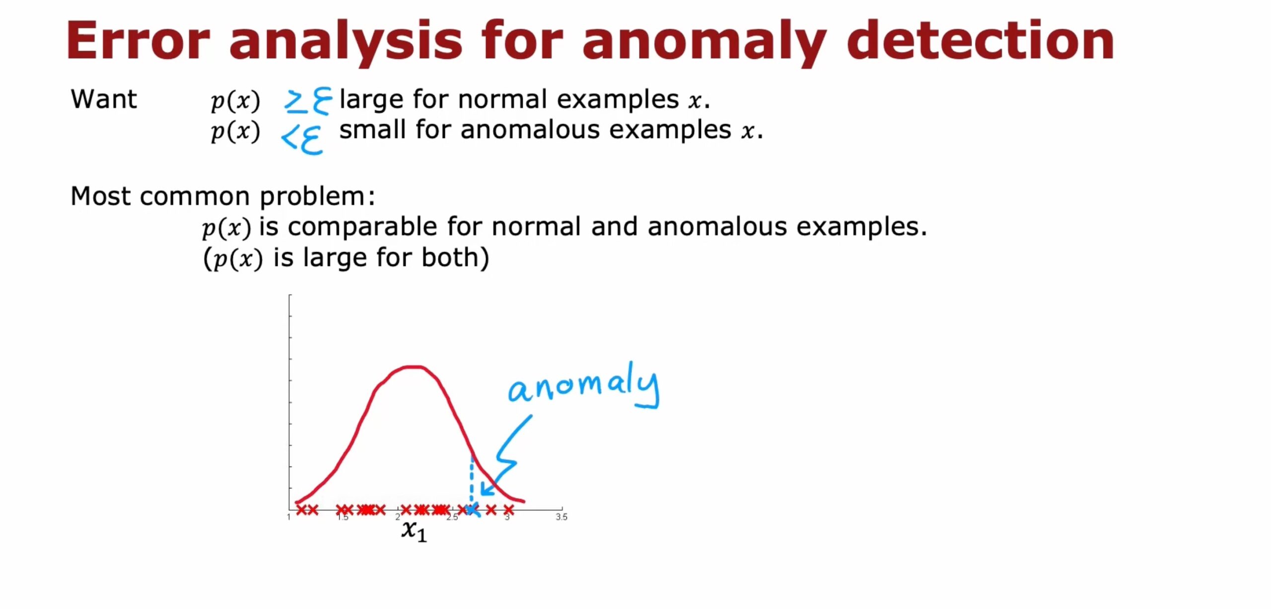
Anomaly detection usually introduces another value:
ε
pronounced:
epsilon
It is the anomaly threshold.
The rule is:
If p(x) < ε
    anomaly
Otherwise:
If p(x) >= ε
    normal
So:
p(x) < ε  → anomaly

p(x) >= ε → normal
The process looks like this:
New value x
     |
     v
Calculate p(x)
     |
     v
Is p(x) < ε ?
   /       \
 YES       NO
  |         |
Anomaly   Normal
This is the basic idea of Gaussian anomaly detection.
14. Practical Example: Server Monitoring
Suppose we monitor:
x1 = CPU usage
x2 = Memory usage
Normal observations:
CPU      Memory

42%       51%
45%       55%
48%       53%
46%       57%
44%       52%
Then suddenly we see:
CPU    = 99%
Memory = 98%
These values are far from the normal range.
Therefore their probability density may be very low.
The system can flag:
Possible anomaly
Gaussian anomaly detection can be used for:
- Fraud detection
- Server monitoring
- Network intrusion detection
- Manufacturing defects
- Sensor failures
- Financial transactions
- Cybersecurity
- Equipment monitoring
15. Multiple Features
Real-world anomaly detection usually has multiple features.
For example:
x1 = CPU usage
x2 = RAM usage
x3 = Disk usage
x4 = Network traffic
x5 = Response time
For each feature we estimate its own mean and variance:
x1 → μ1, σ1²

x2 → μ2, σ2²

x3 → μ3, σ3²

x4 → μ4, σ4²

x5 → μ5, σ5²
Then a simple Gaussian anomaly detector combines them:
p(x) = p(x1) × p(x2) × p(x3) × ... × p(xn)
Or more compactly:
p(x) = Π p(xj)
where j goes from 1 to n.
Then:
If p(x) < ε
    anomaly
Otherwise:
normal
16. The 68–95–99.7 Rule
Gaussian distributions have a useful rule.
Approximately:
68%
of the data lies within:
μ ± 1σ
Approximately:
95%
lies within:
μ ± 2σ
Approximately:
99.7%
lies within:
μ ± 3σ
Visual idea:
                    μ
                    |
              ______|______
            /       |      \
          /         |        \
________/___________|__________\________

      -3σ -2σ -1σ   μ   +1σ +2σ +3σ

            <--- 68% --->

        <------ 95% ------>

    <--------- 99.7% --------->
This also helps explain anomalies.
A point that is many standard deviations away from the mean is usually much less common.
17. m Versus m – 1
You may see two variance formulas.
For anomaly detection:
σ² = (1 / m) × Σ(x(i) - μ)²
In statistics classes you may also see:
s² = (1 / (m - 1)) × Σ(x(i) - x̄)²
The first is commonly used as the maximum-likelihood estimate for Gaussian variance.
The second is commonly used for unbiased sample variance.
For large datasets, the difference between:
1 / m
and:
1 / (m - 1)
is usually very small.
For basic Machine Learning anomaly detection, using:
1 / m
is perfectly reasonable.
18. Gaussian Distribution in Python
import numpy as np

X = np.array([10, 12, 13, 14, 16])

mu = np.mean(X)
variance = np.var(X)
sigma = np.std(X)

print("Mean:", mu)
print("Variance:", variance)
print("Standard deviation:", sigma)
Output:
Mean: 13.0
Variance: 4.0
Standard deviation: 2.0
So:
np.mean(X) → μ

np.var(X)  → σ²

np.std(X)  → σ
19. The Entire Concept in One Picture
                       NORMAL
                          ↓
                         μ
                         |
                    *****|*****
                 ***     |     ***
               **        |        **
             **          |          **
___________**____________|____________**________
     ↑                                         ↑

   Low p(x)                                  Low p(x)
     ↓                                         ↓

Possible anomaly                         Possible anomaly
The important idea is:
Near μ
→ high p(x)
→ common
→ probably normal
while:
Far from μ
→ low p(x)
→ unusual
→ possible anomaly
20. Quick Reference Table
| Concept | Symbol | Meaning |
|---|---|---|
| Mean | μ | Center |
| Standard deviation | σ | Spread |
| Variance | σ² | Spread squared |
| Probability density | p(x) | How plausible x is |
| Threshold | ε | Anomaly boundary |
| Normal | p(x) >= ε | Expected |
| Anomaly | p(x) < ε | Unusually unlikely |
The most important formulas are:
Mean:

μ = (1 / m) × Σ x(i)
Variance:

σ² = (1 / m) × Σ(x(i) - μ)²
Standard deviation:

σ = sqrt(σ²)
Gaussian density:

p(x) = [1 / (sqrt(2π) × σ)]
       × e^(-(x - μ)² / (2σ²))
Anomaly rule:

p(x) < ε → anomaly
Final Mental Model
You do not need to memorize the Gaussian equation first.
Remember this:
μ = What is normal?

σ = How much variation is normal?

p(x) = How unusual is this new value?

ε = At what point do we call it an anomaly?
So Gaussian anomaly detection is essentially asking:
How far does this new observation differ from the behavior I normally see?
If it lies near the center of the learned distribution, it is probably normal.
If it lies far away and produces a very small p(x), it may be an anomaly.

There are 0 comments